The wavelength belongs to the quantity being compared
Two aerosol optical-depth values can differ partly because they describe different wavelengths. Comparing a ground observation at one channel with a satellite product at another without noting that difference mixes spectral behavior with instrument or sampling differences. AOD is dimensionless, but that does not make its spectral coordinate optional. Keep the wavelength beside every value, just as you would retain an acquisition time beside a changing atmospheric observation or a location beside a ground measurement.
The Ångström relation provides a useful approximation for translating AOD between wavelengths over a declared interval. This article works through an invented positive spectrum and calculates an intermediate value at 550 nanometres. It explains the assumption rather than claiming a new aerosol retrieval or validating a satellite product. Matching the spectral coordinate is one preparation step in a comparison; timing, atmospheric support, quality and uncertainty still need their own treatment before the resulting agreement or disagreement can be interpreted.
1. Define AOD and its spectral dependence
NASA's Deep Blue science description defines AOD through vertically integrated aerosol extinction, representing the scattering and absorption of light by particles through an atmospheric column. It notes that satellite products commonly report a reference wavelength of 550 nanometres. AOD is therefore neither a surface concentration nor an unspecified amount of haze. The same atmospheric column can have different optical depths at different wavelengths because the interaction between light and the particle population is wavelength dependent.
The Ångström exponent describes that wavelength dependence. Under a constant-exponent approximation, AOD at a target wavelength equals AOD at a reference wavelength multiplied by the target-to-reference wavelength ratio raised to the negative exponent. A larger positive exponent produces a steeper decrease toward longer wavelengths. This is a compact spectral model, not a chemical identification algorithm. Preserve which interval supplied the exponent rather than treating it as a universal label that can be moved unchanged across any wavelengths or observation conditions. [1] [2]
2. Estimate the exponent from two positive optical depths
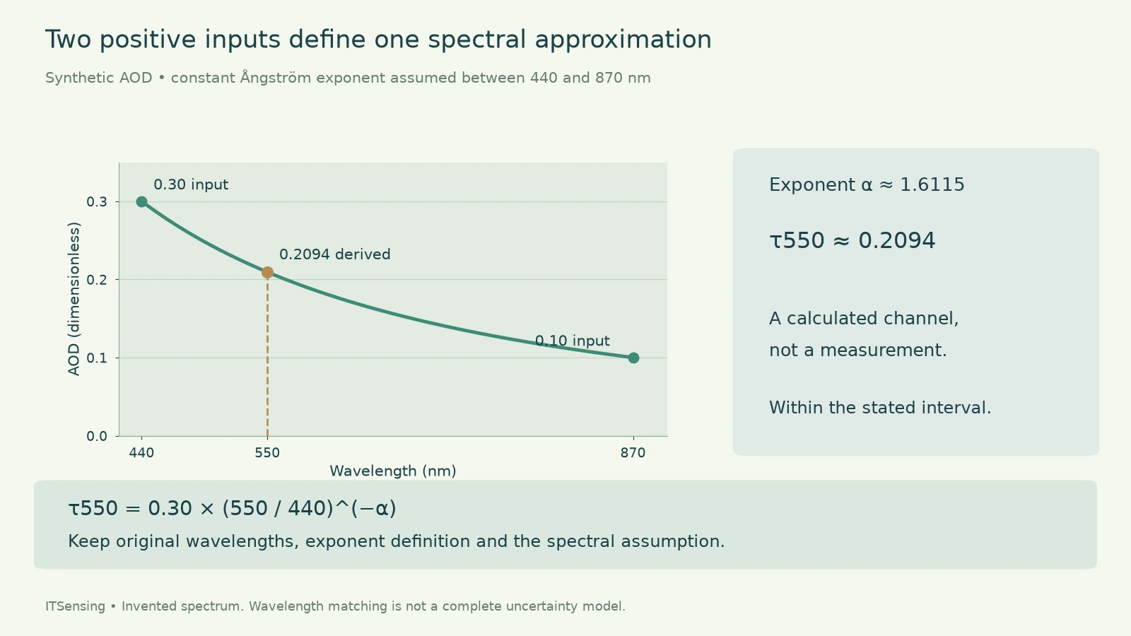
NASA AERONET's explanatory material describes the exponent as the negative slope of optical depth against wavelength in logarithmic coordinates. With two positive AOD values, divide the logarithm of their optical-depth ratio by the logarithm of the longer-to-shorter wavelength ratio. For the invented example, AOD is 0.30 at 440 nanometres and 0.10 at 870 nanometres. The ratio of optical depths is three, while the wavelength ratio is approximately 1.9773.
Using natural logarithms gives an exponent of approximately 1.6115. Using another logarithm base consistently would give the same ratio. The calculation describes the slope between those two spectral points, not proof that the full spectrum is exactly a power law. If the available product supplies an exponent derived from more channels or a different interval, retain its documented definition. Do not silently replace a multichannel estimate with a two-channel calculation and then describe the resulting number as the unchanged original product. [2]
3. Calculate the intermediate 550 nm value
Take the 440-nanometre AOD of 0.30 as the reference. The target-to-reference wavelength ratio is 550 divided by 440, or 1.25. Raise that ratio to minus 1.6115 and multiply by 0.30. Carrying the unrounded exponent through the calculation gives approximately 0.2094 at 550 nanometres. The target lies between the two supplied wavelengths, so this example is an interpolation under the assumed spectral relationship rather than an extrapolation outside the observed interval.
The same result should be obtained using the 870-nanometre point as the reference and the same exponent. That reverse calculation is a useful consistency check on signs and ratios. It does not test whether the atmosphere actually followed the assumed curve, since both calculations use the same fitted relation. Label the intermediate value as calculated and retain the two input observations. A smooth plotted curve can otherwise make an unmeasured wavelength appear to have the same evidential status as the original measurements.
4. Keep wavelength units and spectral support consistent
Both wavelengths in a ratio must use the same length unit. The ratio of 550 to 440 nanometres is identical to the ratio of 0.55 to 0.44 micrometres. Combining a numerical value in nanometres with one in micrometres would create a large artificial discrepancy. Store wavelength values with units and use a reproducible conversion rather than relying on an unlabeled spreadsheet header. The exponent itself remains dimensionless because it relates logarithms of ratios.
Also distinguish a product's nominal reference wavelength from the detailed spectral response used by an instrument or retrieval. The simple calculation here operates on declared AOD wavelengths; it is not a convolution through a sensor's response function. If a validation method specifies a particular spectral conversion, follow its definitions and preserve them in the matchup record. Spectral curvature or a changing particle mixture can limit a constant-exponent approximation, especially when transferring it beyond the interval from which it was estimated.
5. Apply the logarithmic model only to suitable inputs
A logarithmic ratio requires positive input optical depths and distinct positive wavelengths. Zero or negative supplied values cannot be inserted into this particular calculation as though their logarithms were ordinary numbers. Keep the original retrieval values and quality information, then decide through a documented analysis policy which observations support the spectral model. Adding an arbitrary small positive constant to make the equation run changes the data and can strongly affect the estimated exponent at low optical depth.
Small differences between low-loading observations can also make a spectral estimate sensitive to measurement uncertainty. Report sensible precision and inspect the input channels rather than interpreting every exponent fluctuation as a changed aerosol type. This article sets no universal rejection threshold or minimum loading. Such criteria depend on the source product, uncertainties and study design. An unavailable spectral estimate should remain unavailable when its prerequisites are unmet, while any alternative estimator needs its own explicit assumptions and evaluation.
6. Harmonize the remaining observation context
After matching wavelengths, check whether the ground and satellite observations refer to sufficiently comparable times and atmospheric conditions. A point-based ground instrument and a satellite retrieval footprint have different spatial supports. Preserve the averaging window, surrounding variability, valid sample count and the product's quality criteria. A wavelength-adjusted number should not hide a cloud-affected input or a rapidly evolving plume. Harmonization should make a comparison interpretable, not remove every visible disagreement by adding undocumented corrections.
Keep the scientific target separate as well. NASA's aerosol explanation distinguishes column AOD from particulate mass near the surface. Converting between wavelengths does not add vertical distribution information or transform AOD into a ground-level concentration. Likewise, an exponent associated qualitatively with particle size does not identify a unique source or chemical composition. Use the adjusted optical quantity to address an optical comparison, and obtain the additional observations and modeling appropriate to a different atmospheric or environmental question. [1]
7. Deliver the assumptions with the adjusted value
A useful spectral-comparison table includes original AOD values and wavelengths, target wavelength, exponent definition, quality policy and whether the target lies inside the source interval. Retain the unrounded computational values while presenting precision that fits the evidence. Mark the adjusted value as derived and keep it linked to its source record. That allows another analyst to reproduce the arithmetic and to change the spectral assumption without losing the original observations.
In the invented example, the auditable statement is modest and specific: two positive inputs at 440 and 870 nanometres define a constant-exponent approximation that yields about 0.2094 at 550 nanometres. It is not a measured intermediate channel, a complete uncertainty estimate or an aerosol-source diagnosis. This discipline makes wavelength adjustment useful in remote-sensing research because it resolves one identifiable mismatch while leaving the remaining observational and physical questions available for independent examination.