One mask can produce different patch inventories
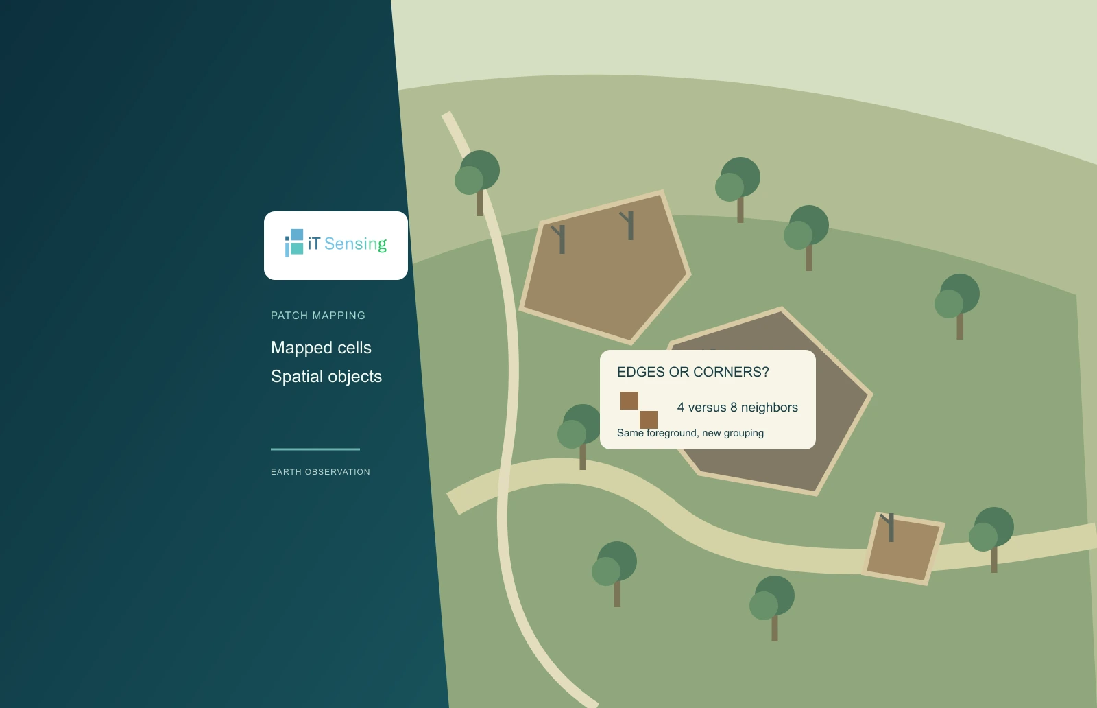
A binary satellite-derived burn mask describes which raster cells meet a declared mapping rule. Turning those cells into a patch inventory adds another decision: what counts as connected. Two foreground cells sharing an edge can be joined under an edge-only rule, while cells meeting at one corner remain separate. A diagonal rule can join them. That small choice can alter the number and size of mapped objects even when no pixel has changed class and the total foreground area is identical.
This tutorial makes that choice visible with a short Python program and an invented mask. It compares four- and eight-neighbor connected components, reports their cell counts and demonstrates how a minimum-size filter interacts with the grouping. It does not detect a real burn, estimate ecological severity or reconstruct the spread of a fire. Its purpose is to help an analyst inspect the spatial rule between a classified raster and the object statistics subsequently delivered to another team.
1. Define the input before labeling objects
The program accepts only a rectangular matrix of zero and one. One means foreground under the chosen burn-mapping definition, while zero is background in this already prepared example. A real multivalued severity raster must first be interpreted using its class definitions. Do not pass every positive class value to this binary routine and assume that all of them mean burned ground. Likewise, unresolved observations need their own documented treatment before a patch inventory can be interpreted across the intended reporting area.
MTBS documentation illustrates why product meaning matters: its burned-area boundaries and incident perimeters are not necessarily interchangeable, and its thematic data contain several classes with different interpretations. The inventory below is an analysis of a declared binary foreground, not an implementation of the MTBS mapping process. Keep the source classification, dates, class-selection rule and observation support beside the derived labels. An object count cannot communicate those choices by itself, however accurately the labeling algorithm runs. [1]
2. Choose the neighborhood deliberately
Four-neighbor connectivity considers the cells immediately above, below, left and right. Eight-neighbor connectivity also includes the four diagonal positions. Both are symmetric relationships: if one cell is considered a neighbor of another, the reverse connection holds. SciPy's labeling documentation demonstrates the distinction through a cross-shaped default structure and a structure that also joins diagonal features. The pure-Python implementation here uses the same neighborhood concepts without requiring SciPy or claiming to reproduce its internal implementation.
Neither rule proves physical continuity on the ground. A corner touch in a categorical raster can arise from sampling, alignment or the shape of a boundary relative to the grid. Choosing eight neighbors does not establish that a continuous strip burned between two mapped cells. Choosing four does not establish that the underlying fire was physically disconnected. Select the neighborhood for the intended mapped-object definition, retain it as a parameter and examine how sensitive the inventory is to that decision. [2]
3. Trace the invented components by hand
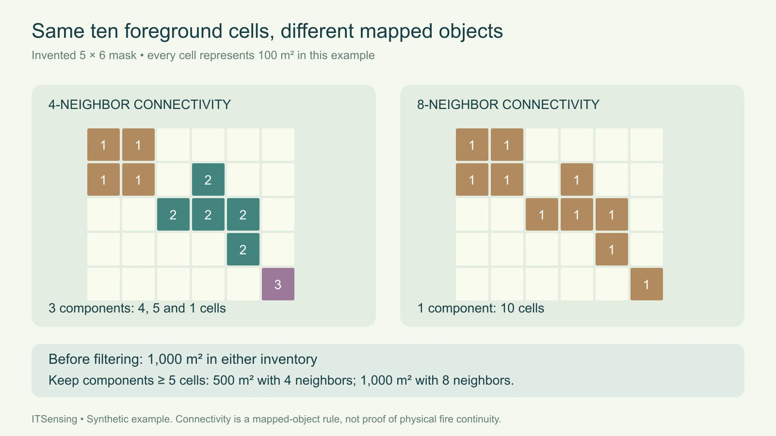
The example mask has five rows and six columns, with ten foreground cells. Its upper-left group contains four cells. A second group, offset down and to the right, contains five edge-connected cells. A final isolated cell lies diagonally beyond the second group. Under four-neighbor connectivity, these form three components with sizes four, five and one. The first group touches the second only diagonally, and the second touches the last cell only diagonally, so neither contact joins them under the edge-only rule.
Under eight-neighbor connectivity, those diagonal contacts create a chain joining all ten foreground cells into one component. The total foreground count remains ten in both runs. With the explicitly assumed cell area of one hundred square metres, both inventories describe one thousand square metres before filtering. This distinction is useful during review: a changed component count need not indicate that the classified area changed. It may simply reflect a different rule for partitioning the same set of foreground cells.
4. Apply minimum-size rules after understanding the grouping
Now retain only components containing at least five cells. With four neighbors, only the five-cell component passes, leaving five hundred square metres in the retained inventory. With eight neighbors, the joined ten-cell component passes, retaining one thousand square metres. The filter threshold is identical, yet its area consequence differs because the objects supplied to it differ. The five-cell threshold is a teaching choice, not a recommended minimum mapping unit for a sensor, ecosystem or monitoring program.
Record the order of operations. Filtering small components, joining nearby objects and changing the input resolution are different operations and need not produce equivalent results in a different sequence. Preserve the unfiltered labels and counts when a filtering decision affects a reported statistic. Otherwise a reviewer may interpret excluded mapped pixels as evidence of an absence on the ground, when the workflow merely removed their components under an analyst-selected size rule.
5. Run the connected-component calculation
Save the code as burn_components.py, run its self-test and then provide a JSON file containing the binary mask, equal cell area and minimum component size. The function visits each foreground cell, starts a new label when necessary and follows allowed neighbors until that component is complete. It returns a label matrix, component counts, areas, total foreground area and the area retained by the size filter. The example runs both neighborhood choices so their consequences can be compared directly.
Inspect a known edge contact, a diagonal contact and an isolated cell in the output. Check that the summed component counts equal the number of input ones and that their total area agrees with the declared cell area. The program rejects ragged rows, nonbinary values, unsupported connectivity and invalid area or size inputs. It is an in-memory teaching implementation for small masks; a large raster workflow needs suitable storage and processing tools rather than an assumption that a small JSON example scales to every scene.
"""Label a prepared binary mask; this does not classify a real burn."""
from collections import deque
import json
import math
import sys


def components(mask, connectivity, cell_area_m2, min_pixels=1):
    if not mask or not mask[0] or any(len(row) != len(mask[0]) for row in mask):
        raise ValueError('Use a nonempty rectangular matrix')
    if any(type(v) is not int or v not in (0, 1) for row in mask for v in row):
        raise ValueError('Mask values must be integer zero or one')
    if type(connectivity) is not int or connectivity not in (4, 8):
        raise ValueError('Connectivity must be 4 or 8')
    if (type(cell_area_m2) not in (int, float) or
            not math.isfinite(cell_area_m2) or cell_area_m2 <= 0):
        raise ValueError('Cell area must be positive and finite')
    if type(min_pixels) is not int or min_pixels < 1:
        raise ValueError('Minimum size must be a positive integer')
    rows, cols = len(mask), len(mask[0])
    labels = [[0] * cols for _ in range(rows)]
    offsets = [(-1, 0), (1, 0), (0, -1), (0, 1)]
    if connectivity == 8:
        offsets += [(-1, -1), (-1, 1), (1, -1), (1, 1)]
    patches = []
    for r in range(rows):
        for c in range(cols):
            if mask[r][c] == 0 or labels[r][c]:
                continue
            label = len(patches) + 1
            labels[r][c] = label
            queue, count = deque([(r, c)]), 0
            while queue:
                y, x = queue.popleft()
                count += 1
                for dy, dx in offsets:
                    ny, nx = y + dy, x + dx
                    if (0 <= ny < rows and 0 <= nx < cols and
                            mask[ny][nx] == 1 and labels[ny][nx] == 0):
                        labels[ny][nx] = label
                        queue.append((ny, nx))
            patches.append({'id': label, 'pixels': count,
                            'area_m2': count * cell_area_m2,
                            'retained': count >= min_pixels})
    return {'connectivity': connectivity, 'labels': labels,
            'component_count': len(patches), 'components': patches,
            'foreground_area_m2': sum(p['area_m2'] for p in patches),
            'retained_area_m2': sum(p['area_m2'] for p in patches if p['retained'])}


EXAMPLE = [[1, 1, 0, 0, 0, 0], [1, 1, 0, 1, 0, 0],
           [0, 0, 1, 1, 1, 0], [0, 0, 0, 0, 1, 0], [0, 0, 0, 0, 0, 1]]


if __name__ == '__main__':
    if sys.argv[1:] == ['--self-test']:
        result = {str(n): components(EXAMPLE, n, 100, 5) for n in (4, 8)}
        assert [p['pixels'] for p in result['4']['components']] == [4, 5, 1]
        assert result['8']['component_count'] == 1
        assert result['4']['retained_area_m2'] == 500
        assert result['8']['retained_area_m2'] == 1000
        print(json.dumps({'passed': True, 'results': result}, indent=2))
    elif len(sys.argv) == 2:
        with open(sys.argv[1], encoding='utf8') as handle:
            data = json.load(handle)
        print(json.dumps({str(n): components(data['mask'], n, data['cell_area_m2'],
                         data['min_pixels']) for n in (4, 8)}, indent=2))
    else:
        raise SystemExit('Use --self-test OR mask.json')
Commands and inventory structure (replace every example input):
python burn_components.py --self-test
python burn_components.py mask.json

mask.json (invented binary mask and 100-square-metre equal-area cells):
{"mask":[[1,1,0,0,0,0],[1,1,0,1,0,0],[0,0,1,1,1,0],[0,0,0,0,1,0],[0,0,0,0,0,1]],"cell_area_m2":100,"min_pixels":5}
6. Keep grid and tile choices in the interpretation
Connectivity belongs to a particular grid. Resampling, moving the grid origin or changing the class boundary can create or remove a corner contact. Reassess patch statistics when those inputs change instead of attributing every difference to the environment. If processing tiles independently, also handle connections across their borders: otherwise one component crossing a seam can be counted as two. A label number assigned during a single scan is not a stable cross-date object identifier, so temporal tracking requires an explicit matching procedure.
When converting the result to vectors, keep the intended connectivity consistent with the polygonization step. GDAL's documentation distinguishes edge-touching from diagonally connected regions. Inspect representative corner contacts and the receiving format's geometry behavior rather than assuming that a raster label guarantees the desired polygon structure. Deliver the binary definition, grid, neighborhood, component table and filtering rule together. That makes the patch inventory reproducible while leaving the physical interpretation of the mapped burn pattern attached to independent evidence. [3]