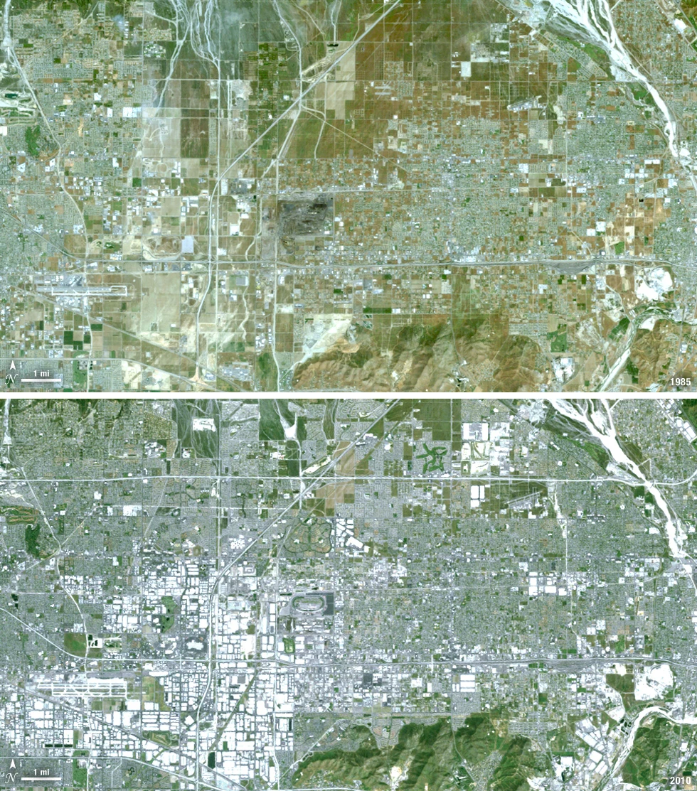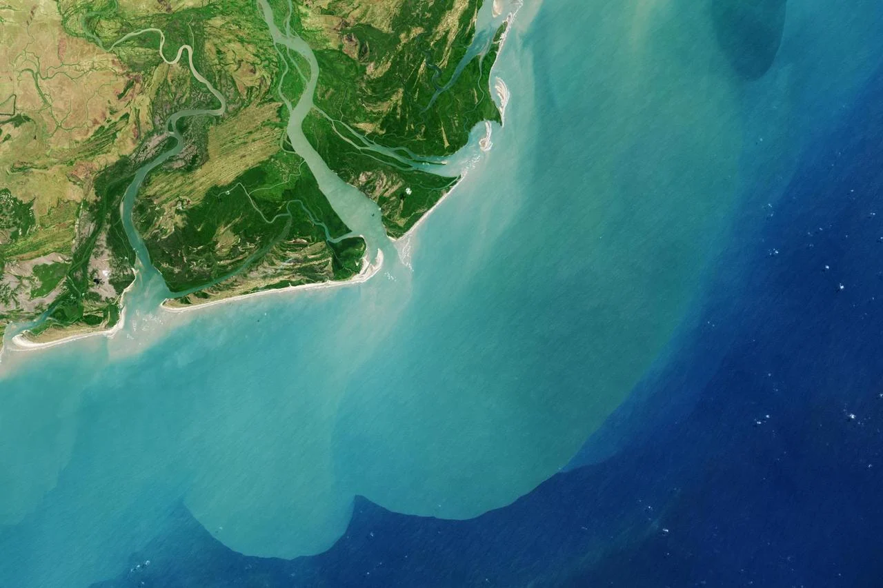
The monitoring question and reporting unit
This implementation guide considers Raster Alignment in the context of Coastal aquaculture ponds, with Landsat 8–9 Collection 2 surface temperature as the selected data source. The purpose is to design a defensible monitoring workflow before purchasing imagery, selecting software settings or committing to an operational alert. Treat the proposed combination as a starting point for a feasibility assessment: the landscape may contain features that the product cannot resolve, and the relevant physical variable may differ from the decision a manager wants to make. Establish that relationship explicitly, then document what additional observations are required.
Landscape context and independent observations
Coastal pond monitoring should distinguish pond boundaries, water presence, exposed bottoms and surrounding vegetation before interpreting operational change. Satellite observations may identify changes needing a field visit, but an optical water pattern does not directly establish stocked species, animal health, feed efficiency or whether a pond meets its production or environmental objectives. Define the reporting unit, the observed variable and the action a finding could trigger before selecting an indicator. Retain these definitions so evaluation addresses the management question rather than visual appearance.
Filling, draining, pond preparation, water exchange and seasonal rainfall can cause strong differences between dates without indicating failure. Narrow dikes and small ponds often mix within a pixel. Retain a pond inventory and management calendar, separating stable boundary geometry from the changing water condition that each acquisition happens to observe inside the pond. Record the observation window and comparison population. Consistent processing cannot compensate for dates or spatial units representing different processes. Preserve acquisition and context information so another analyst can reconstruct the comparison.
Pond color can respond to algae, sediment, dissolved material, depth and illumination. A greener pond is not automatically more productive, and a dark radar response does not prove favorable water quality. Optical or radar contrasts should therefore be treated as surface observations whose connection to husbandry or water chemistry requires local measurements and independent evaluation. Treat competing explanations as hypotheses to test, with insufficient evidence retained as a legitimate result. Avoid forcing every difference into a problem class. Identify the additional observation that would change the interpretation.
Use independent pond observations recording water condition, management stage and sampling time; add laboratory or production measurements when those are the target variables. Deliver pond-level summaries with mixed-edge exclusions and confidence. Clearly distinguish a detected surface change from a biological or chemical diagnosis so farm managers can choose the appropriate follow-up rather than an unsupported treatment. Document reference selection and independence from threshold or model tuning. Preserve usable coverage and rejected observations. State the conclusion's spatial and temporal support so later updates remain comparable without overstating measured evidence.
Select the measurement and data product
The Landsat Collection 2 surface-temperature product estimates the temperature of the radiating surface using thermal observations and auxiliary information. Its delivered raster grid must not be confused with the native resolving power of the thermal measurement. It can reveal broad thermal contrasts between land-cover types, but it is not a direct measurement of shaded air temperature at a weather station.
Convert stored values to Kelvin with the documented scale and offset before deriving Celsius or comparing dates. Retain the product uncertainty and cloud-distance information where supplied, and check whether the scene actually contains a valid temperature layer. Missing auxiliary emissivity information can create persistent gaps. Report those gaps as unavailable observations rather than interpolating them silently into a convincing heat map.
Compare acquisitions with attention to season, local overpass conditions, surface moisture and cloud contamination. A hotter pixel may reflect different materials, water availability or illumination rather than a new operational problem. For local heat planning, combine the raster with land cover and independent temperature observations. Describe the relationship between surface temperature and human heat exposure as an interpretation requiring additional evidence.
Prepare and test the analysis
Verify grid origin, cell size, coordinate system and extent before subtracting rasters. Equal nominal resolution alone does not establish that corresponding cells cover the same area on the ground. Define the decision unit, observation period and consequence of an incorrect result before choosing processing settings. Separate the physical measurement from the management interpretation. The workflow should explain when available imagery is adequate, when more observations are needed, and who is responsible for reviewing uncertain cases.
Select a documented reference grid, transform other inputs once and inspect coincident pixel boundaries. Preserve masks during alignment and distinguish a georeferencing correction from changing the assigned coordinate-system label. Keep a small representative test area and retain the original inputs. Record the product identifier, processing level, coordinate reference system and every setting that changes the numbers. Change one assumption at a time so that a reviewer can distinguish a processing effect from a real difference on the ground.
Two hypothetical 10 metre grids offset by 5 metres sample different footprints. A subtraction along a sharp land-cover edge can therefore show change even when neither surface changed. This is an illustrative calculation for checking the logic, not a measured outcome or a universal threshold. Repeat it on known inputs before processing the full region. Then vary the relevant assumption and document whether the decision changes, including cases where the available evidence cannot support a confident answer.
Repeated reprojection smooths continuous data and may shift categorical boundaries. Forcing an inappropriate coordinate system can also introduce distorted area calculations or apparent displacement mistaken for a sensor problem. A plausible color pattern alone cannot resolve these competing explanations. Review representative failures alongside apparently successful locations, and compare observations made under similar conditions. Preserve a separate uncertainty or exclusion layer so that unsupported areas cannot quietly enter summaries as if they had the same evidential strength as reliable observations.
Test stable edges and independent control locations across the analysis region. Set positional tolerances relative to target size and quantify whether residual misalignment materially changes the final statistics. Set the acceptance rule before examining the final map. Use independent evidence that represents the difficult conditions as well as the easy ones. Report how many observations passed, which failed and why. A threshold that works in this test area still needs checking before transfer to another landscape or season.
Record the reference transform, target grid, transformation method and resampling choices. Keep the aligned outputs separate from source files and include a reproducible description of how alignment was checked. Package the analytical layer with its quality information and a short reproduction note. Include the acquisition dates, processing assumptions, limitations and responsible reviewer. Preserve stable identifiers across maps and tables so another analyst can trace a reported number back to its inputs and repeat the comparison without guessing the settings.
Interpret the combined evidence
Read the landscape and product sections together before applying the analysis procedure. In this guide, Coastal aquaculture ponds defines the reporting context, while Landsat 8–9 Collection 2 surface temperature defines the available measurement; Raster Alignment supplies the processing and review question. These roles are deliberately separate. A working data connection does not establish that the measurement answers the management question. Reject a combination when the target is smaller than the effective observation scale, when the required season has no usable observations, or when the relevant property is not measured by the sensor. Retain that rejection in the project record so that an attractive demonstration does not become an unsupported operational promise.
Acceptance checks before delivery
Write acceptance conditions before inspecting the final map. Specify the reporting boundary, observation period, minimum valid coverage, reference sampling design and the consequence of an incorrect alert. Use project-specific values agreed with the recipient rather than copying a threshold from an unrelated landscape. Keep a small set of independent observations outside all parameter selection. Review omission and commission errors separately and examine boundary areas, rare conditions and missing dates. If the available reference observations do not cover the intended operating conditions, narrow the stated scope of the result instead of claiming that an apparently successful demonstration proves general reliability.
A useful GIS delivery contains more than a colored image. Export the analytical values where licensing permits, the validity mask, reporting geometries with stable identifiers, and a concise record of product names, acquisition dates, processing versions, coordinate reference system and resampling choices. Distinguish valid zero values from missing observations. Provide the area or count of usable measurements for every reporting unit and explain which units were excluded. A colleague should be able to trace a suspicious statistic back to the underlying observation without reconstructing the entire project from screenshots. Store the interpretation and its limits beside the data, not only in a presentation.
Connect the result with an ITSensing workflow
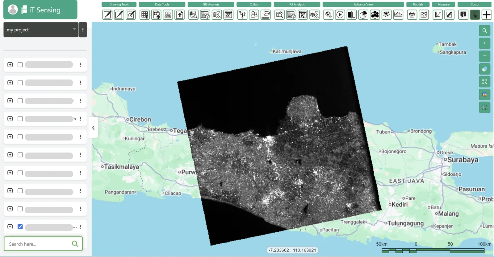
Use the ITSensing satellite catalog and remote sensing tools to evaluate the parts of this workflow that are available for the selected account and data source. Begin with a small representative area and compare the output with a trusted reference before scaling up. The product links below lead to the catalog, tools, documentation and plans so the team can check data access and processing requirements directly. This guide describes an analytical procedure; it does not assert that every named product, algorithm or export format is supplied natively by ITSensing. Where a step uses an external GIS or specialist tool, keep its inputs and outputs in the same reproducibility record.