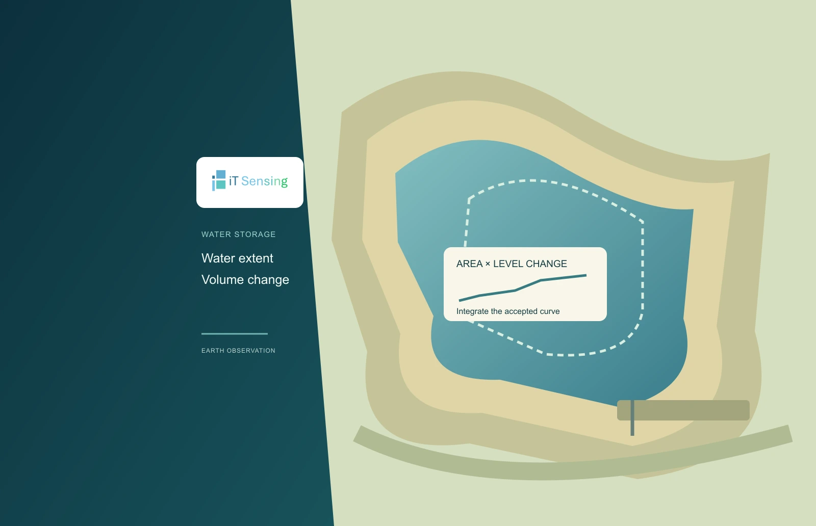
A changing shoreline is not yet a volume estimate
Satellite water outlines can show that a reservoir expanded or contracted, but a change in square kilometres is not a change in cubic metres. A volume calculation also needs information about elevation and the geometry relating area to water level. This tutorial starts with already reviewed area–elevation pairs and integrates a simple curve between two levels. The result is a storage difference under an explicit interpolation assumption, not a claim to know the entire volume hidden below the lowest observed water surface.
The example is intentionally synthetic and uses only the Python standard library. It does not download imagery, retrieve radar heights or infer bathymetry from a photograph. Its value is that every input, unit conversion and integration interval can be inspected. A reader can use the small calculation to review a proposed workflow before connecting it to real satellite observations, gauge records or an independently surveyed capacity curve. Those observations still need their own quality and compatibility assessment.
1. Build a compatible area–elevation record
Each pair must refer to the same water body, an identified vertical reference and a consistent area definition. Match the surface-area observation with the corresponding water level rather than combining a wet-season outline with an unrelated low-water height. Keep acquisition dates, quality information and any partial coverage visible. A fragmentary observed polygon should not be treated as the whole reservoir merely because a height value exists for that pass. Stable water-body identifiers make those checks easier across revisions.
NASA's SWOT LakeSP documentation describes water surface elevation, area, uncertainty and quality indicators, with storage-change products depending on bathymetric assumptions. Those supplied products have their own definitions and processing. The small program here is a separate teaching calculation, not a substitute implementation of that product. Likewise, heights expressed relative to different datums cannot be combined without reconciliation. A constant vertical offset is harmless only when it applies consistently to the entire curve and both requested endpoint levels. [1]
2. State the geometry assumed between observations
For a level water surface and a fixed basin geometry, the incremental volume associated with a small rise is surface area multiplied by the rise. Integrating area with respect to elevation gives the volume difference. This tutorial assumes area varies linearly between each adjacent pair. The volume of each included slice is therefore the mean of its two endpoint areas multiplied by its elevation thickness. This is exact for the chosen piecewise-linear curve, while remaining an approximation to an actual basin whose shape has not been measured continuously.
Other geometry assumptions produce other formulas. The US Army Corps of Engineers' HEC-HMS documentation, for example, describes a conic approximation when constructing storage from elevation and area. That is not the trapezoidal model implemented here. Do not label different methods equivalent because both accept similar-looking tables. Record the chosen interpolation rule and evaluate whether the observation spacing resolves important shoreline or basin transitions. A sparse table can support a transparent calculation without supporting every detail implied by a smooth plotted curve. [2] [3]
3. Check the synthetic curve and units by hand
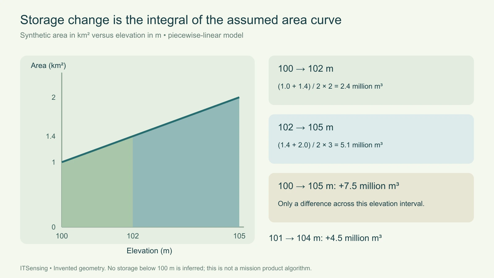
Use invented areas of 1.0, 1.4 and 2.0 square kilometres at elevations of 100, 102 and 105 metres. The first elevation interval is two metres thick, with mean area 1.2 square kilometres. Its volume is 2.4 million cubic metres. The next interval is three metres thick, with mean area 1.7 square kilometres, giving 5.1 million cubic metres. Together they give a storage increase of 7.5 million cubic metres between 100 and 105 metres.
The conversion is essential: one square kilometre multiplied by one metre equals one million cubic metres. Using square kilometres as though they were square metres would understate the result by that factor. An unweighted mean of all three listed areas multiplied by the total level change would also use the wrong integration weights for these unequal intervals. Preserve the individual slice calculations so a reviewer can identify whether a discrepancy comes from units, interval thickness or the assumed curve.
4. Interpolate endpoints without extrapolating the basin
Suppose the requested change is from 101 to 104 metres rather than between listed curve nodes. Linear interpolation gives areas of 1.2 and 1.8 square kilometres at those endpoints. Split the integration at the interior node of 102 metres. The first slice contributes 1.3 million cubic metres and the second contributes 3.2 million, for a total increase of 4.5 million cubic metres. Reversing the endpoints returns the same magnitude with a negative sign, indicating a decrease under the same curve.
The code refuses to extrapolate above or below the supplied elevation range. Observed shoreline geometry at higher levels does not determine the unobserved basin below the lowest level. Report the computed quantity as a difference across the specified interval, not as total stored water at the final elevation. Sedimentation, excavation, changing connections or inconsistent classifications can also undermine a single fixed curve. A decreasing area with increasing level is rejected here as a reason to review the proposed level-pool relationship.
5. Run the calculation and inspect its slices
Save the code as storage_change.py, run its self-test and then supply a JSON file with the curve and two endpoint elevations. The curve must contain finite elevations in strictly increasing order and finite, nonnegative areas that do not decrease. The program preserves that order rather than silently sorting a questionable table. Its output includes the signed volume difference and each positive-thickness slice used before applying the direction of change. It also checks that both endpoint levels lie within the supported range.
For a real record, first reconstruct one slice independently and confirm the reported cubic-metre magnitude. Check that the same level reference is used in the curve and query, that square-kilometre units are correct, and that the water-body boundary has not been changed between inputs. The numerical validation cannot establish those facts from three columns of values. Retain the original source table and the decisions that produced the accepted curve beside the output.
"""Storage difference under a piecewise-linear area/elevation assumption."""
import json
import math
import sys


def storage_change(curve, start_m, end_m):
    if len(curve) < 2:
        raise ValueError('Provide at least two area/elevation pairs')
    for h, area in curve:
        if not (math.isfinite(h) and math.isfinite(area)) or area < 0:
            raise ValueError('Finite elevations and nonnegative finite areas required')
    for (h0, a0), (h1, a1) in zip(curve, curve[1:]):
        if h1 <= h0 or a1 < a0:
            raise ValueError('Elevations must increase; areas must not decrease')
    if not (math.isfinite(start_m) and math.isfinite(end_m)):
        raise ValueError('Endpoint levels must be finite')
    lower, upper = curve[0][0], curve[-1][0]
    if not (lower <= start_m <= upper and lower <= end_m <= upper):
        raise ValueError('No extrapolation outside the supplied curve')
    low, high = sorted([start_m, end_m])
    slices = []
    total = 0.0
    for (h0, a0), (h1, a1) in zip(curve, curve[1:]):
        left, right = max(low, h0), min(high, h1)
        if right <= left:
            continue
        area_left = a0 + (a1 - a0) * (left - h0) / (h1 - h0)
        area_right = a0 + (a1 - a0) * (right - h0) / (h1 - h0)
        volume = (area_left + area_right) / 2 * (right - left) * 1_000_000
        total += volume
        slices.append({'low_m': left, 'high_m': right,
                       'area_low_km2': area_left, 'area_high_km2': area_right,
                       'positive_slice_m3': volume})
    direction = 1 if end_m >= start_m else -1
    return {'start_m': start_m, 'end_m': end_m,
            'storage_change_m3': direction * total,
            'assumption': 'piecewise-linear area in km2 versus elevation in m',
            'positive_slices': slices}


EXAMPLE = [[100, 1], [102, 1.4], [105, 2]]


if __name__ == '__main__':
    if sys.argv[1:] == ['--self-test']:
        whole = storage_change(EXAMPLE, 100, 105)
        partial = storage_change(EXAMPLE, 101, 104)
        assert math.isclose(whole['storage_change_m3'], 7_500_000)
        assert math.isclose(partial['storage_change_m3'], 4_500_000)
        assert math.isclose(storage_change(EXAMPLE, 104, 101)['storage_change_m3'], -4_500_000)
        print(json.dumps({'passed': True, 'whole': whole, 'partial': partial}, indent=2))
    elif len(sys.argv) == 2:
        with open(sys.argv[1], encoding='utf8') as handle:
            data = json.load(handle)
        print(json.dumps(storage_change(data['curve'], data['start_m'], data['end_m']), indent=2))
    else:
        raise SystemExit('Use --self-test OR curve.json')
Commands and inventory structure (replace every example input):
python storage_change.py --self-test
python storage_change.py curve.json

curve.json (invented elevations in metres and areas in square kilometres):
{"curve":[[100,1],[102,1.4],[105,2]],"start_m":101,"end_m":104}
6. Keep physical uncertainty separate from numerical precision
An exact integral of the assumed linear segments does not eliminate uncertainty in the observed areas or elevations. A small height error across a broad water surface can matter, and cloud-obscured margins or mixed shoreline pixels can change an area estimate. Compare defensible alternative input curves or interval choices when assessing sensitivity. Do not invent confidence limits from the number of decimal places in the result or interpret successful program execution as a validation of satellite measurement accuracy.
Deliver the original observations, common reference, accepted curve, interpolation rule, requested levels and signed slice totals together. Explain which elevations are supported and what additional bathymetry would be required for an absolute capacity assessment. The practical outcome is a reproducible storage-change calculation with clear units and boundaries. It can help analysts question an implausible result before using it in a broader water-balance study, while leaving reservoir operations and engineering decisions attached to their appropriate independent evidence.