Begin with the decision and the observable target
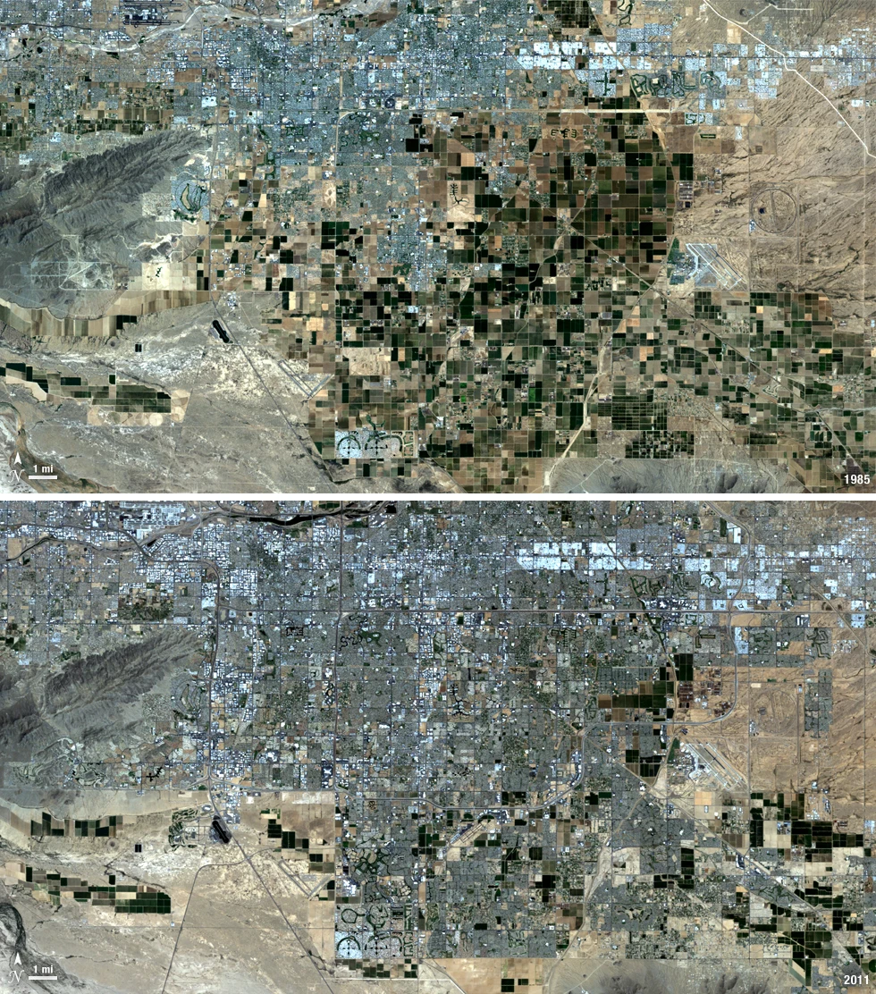
The practical question is: Which irrigation zones repeatedly show conditions that justify a water-delivery review? Work with irrigation management zones as the reporting unit and define the observation period before choosing an image or algorithm. Thermal contrasts, vegetation response and estimated evapotranspiration can reveal spatial differences in surface water use. Interpretation needs crop stage and atmospheric conditions.
Agricultural monitoring works best when the observation unit matches the decision unit. A farmer operates a field, irrigation block or management zone, not an isolated image pixel. Maintain planting dates, crop identity, harvested area and management history in a separate register, then connect the image measurements through stable identifiers. These records explain why neighboring green surfaces may represent different production stages. Before comparing farms, agree on the season definition and the denominator used for every percentage. An area with no usable observation must not silently become bare land, failed crop or normal condition. Review whether the target is large enough for the chosen pixels; field-edge mixtures become especially important in smallholder mosaics. Where the question depends on crop identity, nutrient status, water stress or final production, ask what independent measurement could distinguish competing explanations. The satellite layer should direct that measurement and preserve its outcome. This creates a useful operational record rather than an unexplained color ranking.
Select observations with suitable physical and temporal support
Thermal products require attention to the physical variable and its spatial support. A radiance or brightness-temperature image is not automatically a land-surface temperature estimate, and a land-surface estimate is not air temperature. Use the supplied product definition, scaling, emissivity assumptions and uncertainty flags. Landsat surface-temperature products and ECOSTRESS are examples worth evaluating where their coverage and product properties fit the study. Observation time, cloud contamination, emissivity differences and mixed land cover can influence comparisons. A thermal band resampled to a smaller grid remains limited by its underlying measurement support. Compare locations under sufficiently similar conditions, then test whether the observed contrast survives plausible masking and aggregation choices. Keep the product name, units and acquisition time in the exported attributes so later users can distinguish a measured surface pattern from an inferred process such as crop water use or human heat exposure.
Build a compact data manifest before processing. Record the area of interest, acquisition times, product identifiers, processing versions, bands or variables, units, scale factors and quality criteria. Check the actual usable coverage over the target rather than relying only on scene-wide quality percentages. Preserve the original masks and define how missing values propagate into derived layers. If several dates or sensors are combined, keep their support information available in the project. These details make it possible to repeat a measurement and to explain why a later run changes after a product revision. They also help a colleague decide whether an apparent disagreement comes from the environment, the observation conditions or a processing choice.
Build an analysis rule that can be reviewed
Compare like crops and stages, inspect thermal quality flags and combine temperature anomalies with delivery records. Retain crop-only support area when summarizing each zone.
A predictive relationship needs a clearly defined response variable, reference measurement protocol and intended domain. Standardize units and spatial support before fitting. Reserve genuinely independent samples for evaluation and compare performance with a simple alternative such as the regional mean or a basic physical relationship. Inspect residuals across target range, land-cover context and season; a small overall error can conceal systematic bias in a consequential subgroup. Do not extrapolate beyond the supported range without explicitly evaluating that behavior. Retain measurement uncertainty in the reference data rather than treating every sample as exact truth. Prediction intervals and an out-of-domain mask can be more useful than an extra decimal place. A continuous raster is an estimated surface whose uncertainty needs to travel with the values.
Start with a small, independently reviewed subset before applying the rule across the full geography. Inspect inputs and intermediate layers at both overview and local scales, checking that units, masks and coordinate alignment behave as intended. Keep a named version of the analysis configuration and retain a concise explanation of every consequential threshold. When the workflow moves to another region or season, revisit those assumptions instead of assuming that successful execution proves scientific transfer. A repeatable pipeline is valuable because its choices can be inspected and revised, not because automation makes the interpretation automatically correct.
Interpret the result without hiding alternative explanations
Hot soil between rows can dominate a sparse canopy, and satellite surface temperature is not leaf temperature or a direct irrigation command.
Keep the target interpretation distinct from the evidence used to support it. For irrigation management zones, ask whether the observed pattern persists under a reasonable alternative baseline, quality mask or aggregation. Review apparent successes and plausible counterexamples together. If competing explanations cannot be separated with the available observations, record the finding as a candidate for investigation. This preserves useful spatial information while showing exactly which part of the conclusion still depends on independent evidence. The next observation should be chosen to resolve that uncertainty, rather than simply to reproduce a similar-looking map.
Validate with independent evidence before scaling
Check soil moisture, irrigation timing and representative crop condition during relevant overpasses.
Evaluate estimates with independent measurements that match the spatial and temporal support of the satellite variable. Report bias and error magnitude, inspect residuals across the target range and compare performance with a simple baseline. A model can have a strong correlation while consistently overestimating high values, so correlation alone is insufficient. Where reference measurements have substantial uncertainty, describe that limitation explicitly. Test transfer to the region, season or management context where the output will actually be used. Preserve unsupported contexts as missing or out of domain. If prediction intervals are supplied, assess whether their empirical coverage is appropriate on the independent sample. Keep reference data provenance, units and matching rules with the result so later users understand what the evaluation really tested.
Deliver a usable GIS evidence layer
Provide persistent investigation zones and supporting dates for the irrigation team.
For GIS delivery, retain stable feature identifiers, source observation dates, the physical variable, units, valid support area, uncertainty and review status. Use a suitable coordinate reference for any area or distance calculation and document the transformation when joining outside layers. Separate measured or observed attributes from modeled and field-confirmed attributes so users can update one evidence type without overwriting the others. Include an unknown or unsupported state in summaries and preserve the denominator used for percentages. A map legend, concise data dictionary and accessible source links make the result useful to colleagues who did not run the analysis. Export formats should match the actual downstream workflow, with attribute encoding and geometry checked before handoff.
Turn the method into a practical iT Sensing workflow
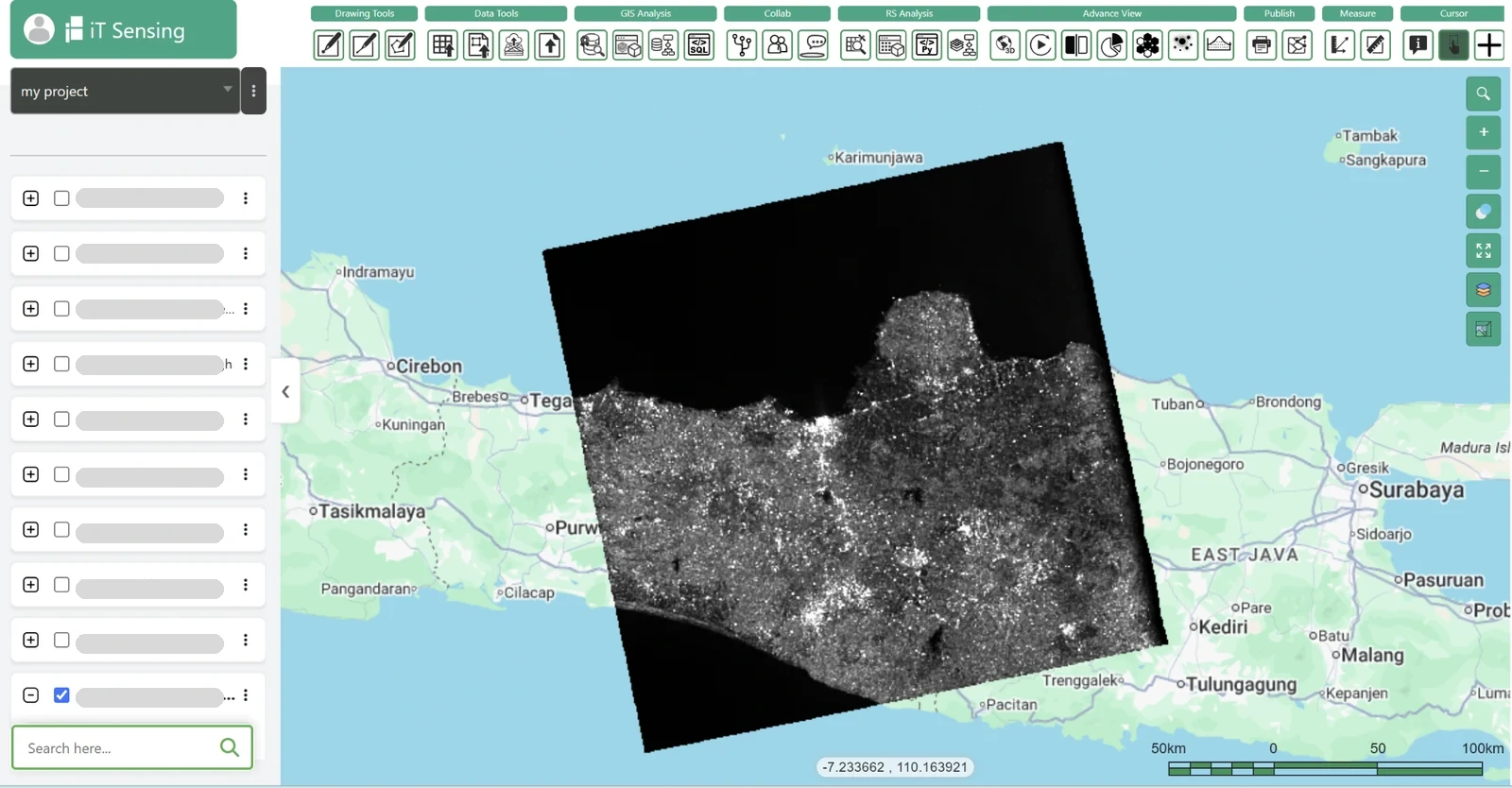
iT Sensing brings satellite discovery, raster analysis, machine learning, GeoAI, visual model workflows and Python experimentation into a cloud remote sensing workspace. Use its documented tools to organize the inputs, test appropriate raster operations and connect evaluated results to a project-aware GIS workflow. The existence of a general tool does not guarantee that every specialist retrieval described here is available as a ready-made operation. Check the documentation and, where necessary, bring independently processed and evaluated products into the project with their provenance intact. A practical next step is to test the workflow on a representative area, review the evidence with domain specialists and choose the workspace plan that fits the team’s real storage, collaboration and processing needs.