Begin with the decision and the observable target
The practical question is: Which coastal reaches show change larger than combined observation uncertainty? Work with coastal monitoring transects as the reporting unit and define the observation period before choosing an image or algorithm. A repeatable land-water or vegetation proxy allows dated coastal positions to be compared along fixed transects.
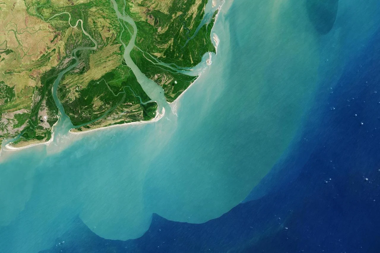
Coastal landscapes change within hours as tides, waves, currents and winds alter the visible surface. Record these conditions when they influence the target. The apparent boundary between land and water is an observation proxy, while habitat extent, administrative coastline and engineering shoreline may require different definitions. Shallow water introduces another complication because the sensor may receive a mixture of water-column and seabed signals. A change in that mixture can reflect depth or clarity rather than ecological change. Compare observations whose environmental context is suitable, and retain incompatible dates for context instead of forcing them into one trend. Offshore products also have spatial support that may be too broad for a small estuary or reef. Preserve this limit in GIS summaries. Coastal mapping becomes more useful when satellite evidence is connected to tide records, habitat observations and local operational histories, with each source still identifiable in the final dataset.
Select observations with suitable physical and temporal support
Optical surface reflectance is a useful starting point for many land-cover questions because it reduces some atmospheric effects before comparison. Landsat and Sentinel-2 are common candidates, but select an actual product whose bands, quality information and spatial support fit the target. Apply the documented scale and offset before interpreting values, and mask cloud, cirrus, shadow and other invalid observations according to the product guidance. A resampled raster does not gain new physical detail: placing a coarser band on a finer grid changes its sampling, not the instrument resolution. Check image alignment near narrow boundaries and use an appropriate common grid for multitemporal work. Review whether the available clear observations cover the biologically or operationally important period. A visually attractive composite can combine dates that do not describe one real state, so retain the contributing acquisition information when timing affects the decision.
Build a compact data manifest before processing. Record the area of interest, acquisition times, product identifiers, processing versions, bands or variables, units, scale factors and quality criteria. Check the actual usable coverage over the target rather than relying only on scene-wide quality percentages. Preserve the original masks and define how missing values propagate into derived layers. If several dates or sensors are combined, keep their support information available in the project. These details make it possible to repeat a measurement and to explain why a later run changes after a product revision. They also help a colleague decide whether an apparent disagreement comes from the environment, the observation conditions or a processing choice.
Build an analysis rule that can be reviewed
Define the proxy, record environmental context and propagate position uncertainty into displacement and rate estimates.
Change detection compares two supported states and must control differences unrelated to the process of interest. Check alignment, product compatibility, seasonal timing and valid observation masks before interpreting a subtraction or transition map. Establish a common comparison area; a cloud-covered location in one date is not a valid zero-change observation. Consider multiple dates to distinguish persistent transitions from a transient image artifact. Thresholds should reflect local variability and independent evidence rather than a visually appealing color break. Inspect small or narrow changes against original observations because modest misalignment can create long false strips. Report the last supported earlier state and first supported later state when exact timing is unknown. Keep the original observations and decision rule so a later reviewer can reproduce the transition.
Start with a small, independently reviewed subset before applying the rule across the full geography. Inspect inputs and intermediate layers at both overview and local scales, checking that units, masks and coordinate alignment behave as intended. Keep a named version of the analysis configuration and retain a concise explanation of every consequential threshold. When the workflow moves to another region or season, revisit those assumptions instead of assuming that successful execution proves scientific transfer. A repeatable pipeline is valuable because its choices can be inspected and revised, not because automation makes the interpretation automatically correct.
Interpret the result without hiding alternative explanations
Tides, waves and seasonal beach state move the visible line without equivalent long-term erosion. Different proxies should not be merged casually.
Keep the target interpretation distinct from the evidence used to support it. For coastal monitoring transects, ask whether the observed pattern persists under a reasonable alternative baseline, quality mask or aggregation. Review apparent successes and plausible counterexamples together. If competing explanations cannot be separated with the available observations, record the finding as a candidate for investigation. This preserves useful spatial information while showing exactly which part of the conclusion still depends on independent evidence. The next observation should be chosen to resolve that uncertainty, rather than simply to reproduce a similar-looking map.
Validate with independent evidence before scaling
Compare independent shoreline surveys and stable reference sections.
Evaluate the timing and persistence of the inferred process as well as its mapped location. Independent observations should bracket the relevant transition where possible, with their own date uncertainty recorded. Avoid treating a field visit long after acquisition as exact truth for the earlier image. Check whether the method performs differently during sparse observation periods or near seasonal transitions. Include apparently unchanged locations in the evaluation, since reviewing only flagged events cannot reveal missed changes or baseline instability. When timing is represented as an interval, assess whether independently known events fall within that interval. Document cases where the reference itself is ambiguous. A defensible temporal evaluation explains both how often a process is detected and how precisely its occurrence can be placed in time.
Deliver a usable GIS evidence layer
Deliver reach-level changes with uncertainty and proxy limitations.
For GIS delivery, retain stable feature identifiers, source observation dates, the physical variable, units, valid support area, uncertainty and review status. Use a suitable coordinate reference for any area or distance calculation and document the transformation when joining outside layers. Separate measured or observed attributes from modeled and field-confirmed attributes so users can update one evidence type without overwriting the others. Include an unknown or unsupported state in summaries and preserve the denominator used for percentages. A map legend, concise data dictionary and accessible source links make the result useful to colleagues who did not run the analysis. Export formats should match the actual downstream workflow, with attribute encoding and geometry checked before handoff.
Turn the method into a practical iT Sensing workflow
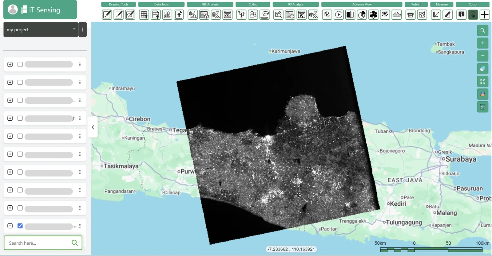
iT Sensing brings satellite discovery, raster analysis, machine learning, GeoAI, visual model workflows and Python experimentation into a cloud remote sensing workspace. Use its documented tools to organize the inputs, test appropriate raster operations and connect evaluated results to a project-aware GIS workflow. The existence of a general tool does not guarantee that every specialist retrieval described here is available as a ready-made operation. Check the documentation and, where necessary, bring independently processed and evaluated products into the project with their provenance intact. A practical next step is to test the workflow on a representative area, review the evidence with domain specialists and choose the workspace plan that fits the team’s real storage, collaboration and processing needs.