The white footprint leaves an important dimension unresolved
A snow-covered mountain basin can look reassuringly full in an optical image while leaving the amount of stored water unresolved. The visible footprint answers where snow is mapped under an observation and classification policy. Water storage also depends on the water equivalent of that snow. A thin layer and a much heavier snowpack can occupy the same horizontal area, so a snow-cover map alone cannot supply the missing vertical water-equivalent dimension, however detailed its boundaries appear.
The distinction becomes especially useful when snow observations enter basin reports or comparisons between seasons. Snow-covered area, snow depth and snow water equivalent should remain separate variables with explicit units and averaging domains. This article follows an invented basin calculation to make those domains visible. It does not estimate a real snowpack, select a universal density or forecast spring runoff. Its goal is to prevent an otherwise correct multiplication from attaching a water volume to the wrong spatial denominator.
Optical snow indices describe a spectral contrast
USGS describes Landsat NDSI as a normalized contrast between green and shortwave-infrared reflectance. Its formula divides their difference by their sum. That ratio is dimensionless; its units are not metres of snow or kilograms of stored water. A snow-mapping workflow can use such spectral information with quality and contextual screening, but the resulting snow footprint remains a different kind of quantity from a water-equivalent depth. Retain the index, mapped class and usable-observation mask distinctly in the analysis.
An image's unobservable terrain also needs its own status. If cloud or unsuitable illumination prevents interpretation, the affected ground is not automatically snow-free. Report the mapped snow area together with the area actually evaluated, and avoid comparing percentages whose support changes silently. A sharper-looking boundary or a different color scale cannot resolve the water content beneath the optical surface. Additional observations and a physical estimation framework are needed when the reporting question concerns storage rather than the presence of snow. [1]
Snow depth and water-equivalent depth are different lengths
NSIDC defines snow water equivalent through the water content obtained by melting the snowpack. USACE's snow-properties reference relates SWE to snow depth through the ratio of depth-averaged snow density to water density. Thus two layers of identical physical depth can have different SWE if their average densities differ. The measurement names can both carry length units, yet they describe different substances and cannot be interchanged just because a report column is labeled in millimetres.
For a deliberately simplified illustration, take a half-metre snow layer and use one thousand kilograms per cubic metre as the assumed water density. A snow density of two hundred kilograms per cubic metre gives one hundred millimetres of SWE. Changing the assumed snow density to five hundred gives two hundred fifty millimetres. These are invented inputs for the relationship, not recommended density defaults. No satellite index or snow-covered outline in this example determines which density, depth or water equivalent is present. [2] [3]
Hold the area constant and change the stored water
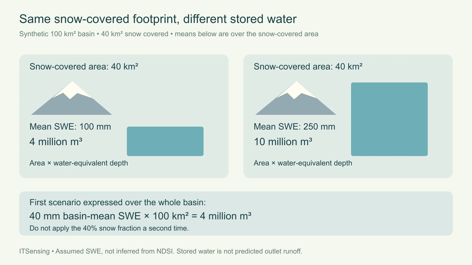
Now imagine a one-hundred-square-kilometre basin in which forty square kilometres are snow covered. Suppose the mean SWE over that snow-covered portion is one hundred millimetres. Convert the area to forty million square metres and the water-equivalent depth to one tenth of a metre. Their product is four million cubic metres of stored water. The calculation assumes that the stated mean really represents the entire covered portion; it is not justified by one convenient point sample alone.
Keep the same forty-square-kilometre footprint but assign a snow-covered-area mean SWE of two hundred fifty millimetres. The stored volume becomes ten million cubic metres. Both scenarios have forty percent snow cover, yet the second stores two and a half times as much water under the declared assumptions. This is a dimensional counterexample, not an observed contrast between two named basins. It shows exactly which missing quantity prevents an optical area map from becoming a standalone storage measurement.
A basin-average SWE must not be multiplied by snow fraction twice
There is another valid way to express the first scenario. Spread its four million cubic metres across the entire hundred-square-kilometre basin, including snow-free ground, and the basin-average SWE is forty millimetres. Multiplying that forty-millimetre depth by the whole basin area recovers the same four million cubic metres. The snow-covered-area mean was one hundred millimetres; the basin-wide mean is forty. Neither is wrong, but each belongs to a different denominator that must remain visible beside the number.
If a dataset already reports an area mean that includes snow-free zero values, multiplying its volume calculation by the snow fraction again would double-apply that fraction. Conversely, multiplying a snow-covered-only mean by the full basin without the fraction would overstate volume. Read the product's variable and aggregation definitions before combining it with a snow mask. Point SWE, a grid-cell mean and a basin aggregate are also different supports; their labels should make clear which is actually being used.
Spatial variability belongs in the storage estimate
For a heterogeneous basin, partitioning into compatible areas can make the integration explicit. Each area's representative SWE contributes its area multiplied by water-equivalent depth, and those volumes are summed. Retain whether the area represents all ground or only its snow-covered part. Keep unknown SWE separate from confirmed zero. A coarse mean can be useful at its intended support, while copying it to a finer display grid does not create independent knowledge of every shaded slope or wind-redistributed drift.
Ground measurements need the same care. A snow sample or station record describes a particular location and time, and its basin representativeness needs evaluation. Pair observations with terrain and acquisition context instead of assuming that a point is the basin mean. When different dates supply the snow footprint and SWE estimate, assess whether accumulation or melt changed the state between them. A table of individually accurate observations can still yield a misleading storage number when their temporal or spatial supports do not agree.
Stored water is one input to a runoff assessment
A calculated snow-water volume is not automatically the volume that will arrive at an outlet or be available for use. USACE distinguishes SWE from snowpack temperature, liquid water content and snow-covered area in its physical description. Those distinctions help explain why a storage snapshot is not a complete melt-and-routing model. The timing of release and what happens after water leaves the pack require further hydrological information. This article supplies no conversion factor from stored snow water to guaranteed downstream supply.
A defensible basin handover therefore reports the snow-map support, SWE definition, averaging domain, units, dates and integration assumptions together. Present uncertainty or unresolved coverage without replacing it with a visually continuous field. Use optical snow extent for the spatial evidence it provides, and use appropriately supported SWE observations or estimates for water-equivalent storage. Keeping both the numerator and the area denominator clear allows a reader to reproduce the volume calculation and recognize the additional evidence needed before interpreting it as a forecast. [3]