Estimate change without hiding the time axis
Satellite observations rarely arrive at perfectly even usable intervals. Cloud screening, acquisition choices and product gaps can leave a time series with several short intervals and a long break. A slope calculation must retain those elapsed times. Replacing them with row numbers changes the rate being estimated, even if the observations remain in the right order. Theil–Sen estimation is a useful way to explore a linear trend, provided its time coordinates, input quality and scientific interpretation remain explicit.
This tutorial implements the estimator's median pairwise slope using Python's standard library. It includes a small invented vegetation-index series with one unusually high middle observation and compares elapsed years with equally spaced row indices. The code is intended for transparent inspection of a short series, not continental raster processing or an automatic change-alert system. It returns a slope, a declared intercept convention and the individual pair slopes so the result can be checked before it enters a monitoring report.
1. Define the input variable and elapsed-time unit
Start with observations of a compatible variable over a consistent spatial support. Retain the original acquisition dates and quality decisions in the project record. Convert dates to a documented numerical elapsed-time coordinate before using this function; the example directly supplies elapsed years. The code does not parse calendar dates or decide how a calendar year should be represented. Its output rate is expressed per unit of the supplied coordinate, which is why the input includes an explicit time-unit label.
Missing or rejected observations require an upstream policy rather than a silent numerical substitution. This implementation rejects null and nonfinite values, repeated times and observations that are not in strictly increasing time order. It does not fill gaps, clip an index range or remove unusual points automatically. A robust estimator is not a substitute for screening known invalid retrievals. Keep valid extreme observations distinct from documented sensor or processing failures, and preserve the reason for any exclusion before fitting the series.
2. Form all pairwise rates and take their median
For each earlier observation and each later observation, divide their value difference by their elapsed-time difference. The Theil–Sen slope is the median of those pairwise rates. SciPy's official documentation describes that estimator and distinguishes alternative intercept conventions. Here the intercept is the median of each observed value minus the estimated slope multiplied by its time coordinate. This is the documented joint convention, chosen explicitly rather than presented as the only possible definition of a Theil–Sen intercept.
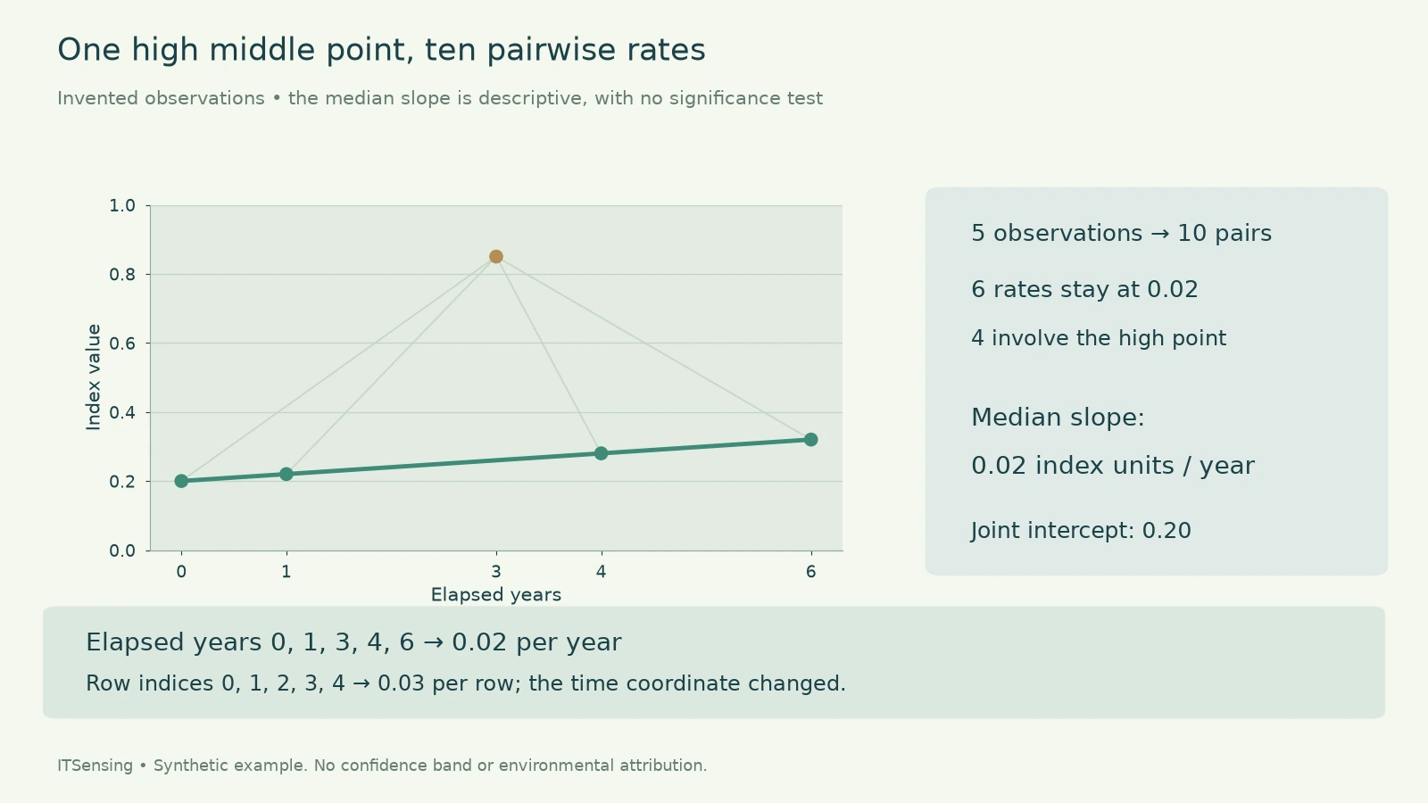
Five observations produce ten distinct earlier-later pairs. A single unusual observation participates in four of them, while the remaining six connect the other observations. This pair structure helps explain the result of the invented example, but it is not a promise that arbitrary contamination will leave the slope unchanged. Which points are unusual, their placement and the rest of the data all matter. Inspect the time series and residual pattern instead of treating a robust method's name as a universal guarantee. [1]
3. Trace the five-observation example
The example uses elapsed years zero, one, three, four and six, with invented index values 0.20, 0.22, 0.85, 0.28 and 0.32. Four observations lie on a line starting at 0.20 and increasing by 0.02 index units per year. The middle value at year three is deliberately raised. Pairing only the four points on the line gives six rates of 0.02. The four rates involving the high middle observation include both positive and negative departures from that value.
Taking the median of all ten rates gives 0.02 index units per year, and the chosen joint intercept is 0.20. The high point remains visible in the input and output; it has not been deleted by an undocumented rule. This is a synthetic arithmetic demonstration rather than a recovered trend from a real satellite site. An index rate also retains its own meaning: a change of 0.02 index units per year does not automatically mean a two-percent annual increase in biomass, yield or ecological condition.
4. Compare elapsed years with row indices
Now keep the same five values but replace the times with zero, one, two, three and four. The median pairwise slope becomes 0.03 per row step. That result is not the same physical rate with a different display label; the uneven intervals have been replaced by an equal-spacing assumption. The six-year span was compressed into four row steps, and individual interval lengths changed. Reporting the row-based result as index units per year would therefore give the calculation a time meaning it did not use.
This distinction matters after filtering a series. Removing a cloudy year must not cause every later observation to move one year earlier in the slope calculation. Keep the remaining observations' original time coordinates. Likewise, monthly and annual summaries require their own consistent timing definitions and should not be mixed through a convenient sequence index. If the analytical target changes from individual acquisitions to seasonal summaries, document that aggregation and its temporal support before interpreting a difference between the two fitted rates.
5. Run the code and inspect its pair table
Save the implementation as sen_slope.py and the example JSON as series.json. Run the self-test and then the example command. The result contains observation count, pair count, slope, joint intercept, time-unit label and a table identifying each pair's time difference and rate. The source uses a straightforward double loop so every contribution is visible. Its pair count grows quadratically with the number of observations, making this an explanatory implementation rather than a claim of suitability for every archive size.
Check a short interval, a long interval and a pair spanning the unusual middle point. Confirm that the ten entries refer to the intended observations and that the reported unit is year for this input. Try replacing the times with row indices while labeling that coordinate honestly as a row. The changed result should prompt a review of the question, not a software correction that forces agreement. The program supplies no confidence interval, p-value, breakpoint date or causal attribution.
"""Transparent Theil-Sen slope for a short, already screened time series."""
import json
import math
import statistics
import sys


def finite_number(value):
    return type(value) in (int, float) and math.isfinite(value)


def estimate(times, values, time_unit):
    if not isinstance(times, list) or not isinstance(values, list):
        raise ValueError('Times and values must be lists')
    if len(times) != len(values) or len(times) < 2:
        raise ValueError('At least two paired observations are required')
    if not all(finite_number(v) for v in times + values):
        raise ValueError('Times and values must be finite numbers')
    if any(b <= a for a, b in zip(times, times[1:])):
        raise ValueError('Times must be strictly increasing')
    if not isinstance(time_unit, str) or not time_unit.strip():
        raise ValueError('Declare the elapsed-time unit')
    pairs = []
    for i in range(len(times) - 1):
        for j in range(i + 1, len(times)):
            delta = times[j] - times[i]
            slope = (values[j] - values[i]) / delta
            if not finite_number(delta) or not finite_number(slope):
                raise ValueError('Pair calculation overflowed')
            pairs.append({'earlier': i, 'later': j,
                          'elapsed': delta, 'slope': slope})
    slope = statistics.median(p['slope'] for p in pairs)
    offsets = [y - slope * t for t, y in zip(times, values)]
    if not all(finite_number(v) for v in offsets):
        raise ValueError('Intercept calculation overflowed')
    return {'observations': len(times), 'pair_count': len(pairs),
            'time_unit': time_unit, 'slope_per_time_unit': slope,
            'joint_intercept': statistics.median(offsets),
            'pairs': pairs}


EXAMPLE = {'times': [0, 1, 3, 4, 6],
           'values': [0.2, 0.22, 0.85, 0.28, 0.32],
           'time_unit': 'year'}


def self_test():
    result = estimate(**EXAMPLE)
    rows = estimate(list(range(5)), EXAMPLE['values'], 'row')
    assert result['pair_count'] == 10
    assert math.isclose(result['slope_per_time_unit'], 0.02)
    assert math.isclose(result['joint_intercept'], 0.2)
    assert math.isclose(rows['slope_per_time_unit'], 0.03)
    return {'passed': True, 'elapsed_years': result, 'row_indices': rows}


if __name__ == '__main__':
    if len(sys.argv) != 2:
        raise SystemExit('Usage: python sen_slope.py --self-test | series.json')
    if sys.argv[1] == '--self-test':
        result = self_test()
    else:
        with open(sys.argv[1], encoding='utf-8') as stream:
            result = estimate(**json.load(stream))
    print(json.dumps(result, indent=2, allow_nan=False))
Commands and inventory structure (replace every example input):
python sen_slope.py --self-test
python sen_slope.py series.json

series.json contains invented index observations and elapsed years:
{"times":[0,1,3,4,6],"values":[0.2,0.22,0.85,0.28,0.32],"time_unit":"year"}
6. Interpret the slope alongside seasonality and site history
A straight-line summary can mix seasonal behavior, a disturbance and gradual recovery into one number. If early observations mostly sample a dormant season while later ones sample peak growth, a robust slope still describes that changing sample. Examine observation timing and compare compatible seasonal support or use an explicitly appropriate seasonal model. Serial dependence and repeated measurements also matter for uncertainty analysis; the pair table contains many rates derived from the same observations, not an equivalent collection of independent experiments.
Deliver the fitted rate with its variable definition, observation period, spatial support, retained times and input-screening policy. Plot the observations with the fitted line and investigate whether a linear summary is scientifically useful. A monitoring report can then distinguish a reproducible descriptive slope from evidence about the mechanism behind it. The estimator is valuable because its calculation can be inspected and its sensitivity explored, while the claim about environmental change remains tied to the actual measurements and an appropriate study design.